Example usage

Here we will demonstrate how to use lrasm in a project to check linear regression assumptions:

from lrasm.homoscedasticity_tst import homoscedasticity_test
from lrasm.multicollinearity_tst import multicollinearity_test
from lrasm.normality_tst import normality_test
from sklearn import datasets
import pandas as pd
import matplotlib.pyplot as plt

#print(lrasm.__version__)

/home/docs/checkouts/readthedocs.org/user_builds/lrasm1234/envs/latest/lib/python3.9/site-packages/statsmodels/compat/pandas.py:65: FutureWarning: pandas.Int64Index is deprecated and will be removed from pandas in a future version. Use pandas.Index with the appropriate dtype instead.
  from pandas import Int64Index as NumericIndex

Define Sample Data

We will use the Iris dataset from scikit-learn to demonstrate the functionality of lrasm.

data = datasets.load_iris()
iris_df = pd.DataFrame(data=data.data, columns=data.feature_names)
iris_df

	sepal length (cm)	sepal width (cm)	petal length (cm)	petal width (cm)
0	5.1	3.5	1.4	0.2
1	4.9	3.0	1.4	0.2
2	4.7	3.2	1.3	0.2
3	4.6	3.1	1.5	0.2
4	5.0	3.6	1.4	0.2
...	...	...	...	...
145	6.7	3.0	5.2	2.3
146	6.3	2.5	5.0	1.9
147	6.5	3.0	5.2	2.0
148	6.2	3.4	5.4	2.3
149	5.9	3.0	5.1	1.8

150 rows × 4 columns

In our example, we want to investigate the linear relationship between the response petal width (cm) versus the predictors: sepal length (cm), sepal width (cm), and petal width (cm). We start by splitting the dataset into a dataframe containing the predictors and a series containing the response:

X = iris_df.drop("sepal width (cm)", axis = 1)
X

	sepal length (cm)	petal length (cm)	petal width (cm)
0	5.1	1.4	0.2
1	4.9	1.4	0.2
2	4.7	1.3	0.2
3	4.6	1.5	0.2
4	5.0	1.4	0.2
...	...	...	...
145	6.7	5.2	2.3
146	6.3	5.0	1.9
147	6.5	5.2	2.0
148	6.2	5.4	2.3
149	5.9	5.1	1.8

150 rows × 3 columns

y = iris_df["petal width (cm)"]
y

    0.2
    0.2
    0.2
    0.2
    0.2
      ... 
  2.3
  1.9
  2.0
  2.3
  1.8
Name: petal width (cm), Length: 150, dtype: float64

Test for Homoscedasticity of Residuals

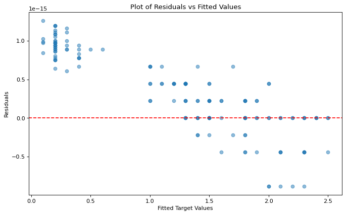
We can evaluate the homoscedasticity of our residuals by passing our predictors and response into the function homoscedasticity_test(). Note that homoscedasticity_test() returns two objects, the first one is a dataframe containing the correlation coefficient of absolute residuals vs predicted values along with the P value of said correlation, while the second is a plot of residuals vs predicted values.

corr_df, plot = homoscedasticity_test(X, y)

The correlation coefficient between the absolute residuals and the fitted y values is:  0.734  With a p value of:  0.0
The p value of the correlation is below the rejection threshold, thus the correlation is likely significant.         
The data is unlikely to be homoscedastic.

corr_df

	correlation_coefficient	p_value
0	0.734	0.0

In the example above, it’s clear that the residuals are not independent of the fitted values, thus we would conclude that the linear relationship is not homosecdastic.

Test for Normality of Residuals

We can evaluate the normality of our residuals by passing our predictors and response into the function normality_test(). Note that normality_test() returns two objects, the first one is a p-value from the Shapiro Wilk test, while the second is a string containing either the word Pass or Fail depending on the results of the test. The function will also print a summary statement.

p_value, res = normality_test(X, y)

After applying the Shapiro Wilks test for normality of the residuals the regression assumption of normality has failed and you should make some djustments before continuing with your analysis

p_value

7.085905963322148e-05

res

'Fail'

In the example above, it’s clear that the residuals are not normaly distributed, and that this assumption has failed.

Test for multicollinearity

We can evaluate the multicollinearity assumption of our data set by passing the features and the threshold for the VIF value. multicollinearity_test() takes these two arguments and returns a data frame with VIF for each feature along with the statement advising the user whether the multicollinearity assumption is violated.

vif_df = multicollinearity_test(X, VIF_thresh = 10)

3 cases of possible multicollinearity
0 cases of definite multicollinearity
Assumption partially satisfied

Consider removing variables with high Variance Inflation Factors

vif_df

	features	VIF
0	sepal length (cm)	15.984946
1	petal length (cm)	95.111245
2	petal width (cm)	49.204035

As we can see above, all VIFs are greater then the pre-defined threshold. That is why we three possible multicollinearity cases.